
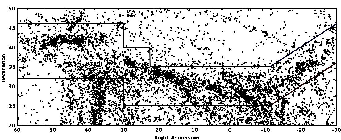
 c. Which figure in the Wegner et al. paper is similar to this figure?
What is different about the one displayed here?
c. Which figure in the Wegner et al. paper is similar to this figure?
What is different about the one displayed here?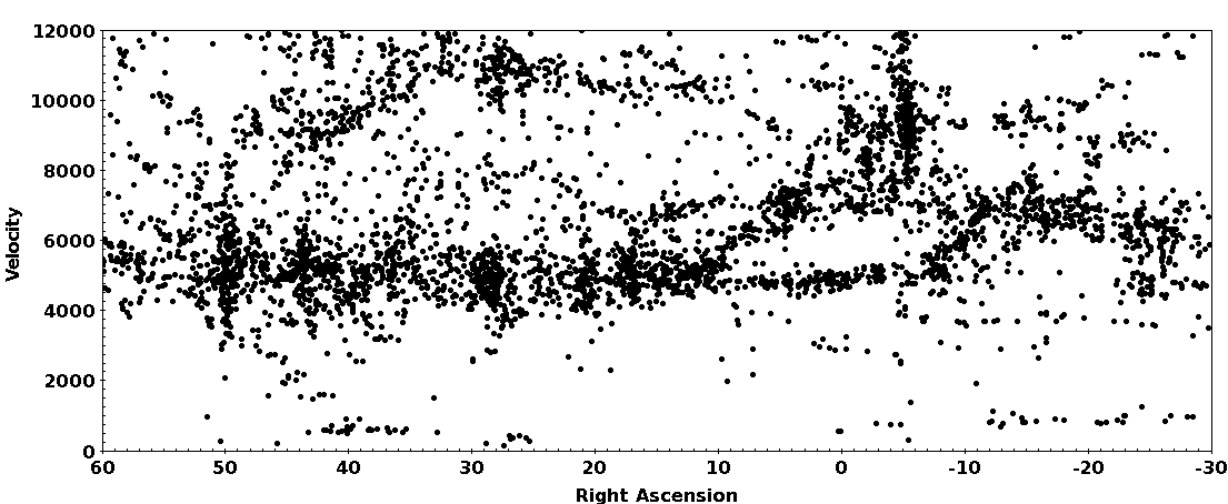 f. What do we mean by "heliocentric velocity"?
1.1 Position-switched observing with single dish telescopes ALFALFA itself was a "blind drift scan" survey in which we positioned the Arecibo telescope on the meridian, pointed it at a particular declination, started taking data and let the sky drift by. For our APPSS observations, we point the telescope towards targets identified by the optical and UV emission. The HI line signals that we are trying to detect are billions of times weaker than the radio noise contributed by the radio receiver, the electronics, the antenna, the cosmic microwave background and the sky overall. So, somehow, we have to subtract off all of those unwanted contributions to find the HI signal from the target galaxy. We can do this by assuming that any random position in the sky does not contain an HI line source at the exact same velocity as our target source and that the difference between the spectra obtained in the direction of our target and some suitably chosen random position will yielf the signal we are after. The mode of observing we use for the L-band wide observations is called position switching, where we switched between "ON source" and "OFF source" positions. Thus each observations is actually on ON/OFF pair of observations. Review with your group the link noted above: L-band wide (LBW) observing for ALFALFA followup. a. What do we mean by system temperature?
b. What is the typical system temperature of the Arecibo L-band receiver system?
c. What is the typical system temperature of the L-band receiver system on the GBT?
d. What is the GBT able to deliver a lower system temperature on its L-band system than Arecibo can?
e. For our Arecibo position-switched observations for APPSS, a source with a a peak flux density of 30 mJy per spectral channel would be easily detected. How does 30 mJy compare with the system temperature you found above?
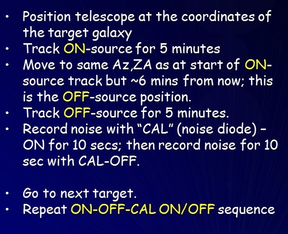
| We also need a way to figure out the intensity calibration of the system noise. To do this, we inject the noise from a diode (whose noise has been measured by the engineers in the lab) into the system and also record the noise when the diode is "off". This sequence is referred to as the "CAL ON/CAL OFF" sequence; we perform this measurement at the end of every target galaxy position-switched ON/OFF pair. A single observation of a target source then includes both the ON/OFF source observation and the CAL ON/OFF calibration sequence, as summarized by the panel to the right. Sometimes, we observe a source more than once, often on a different day, for example, if there is a marginal detection whose reality we would like to confirm. It is possible to combine multiple observations of the same source to improve the signal-to-noise ratio. |
|
1.2 Searching for galaxies using L-band wide You may have noticed that the "spectrometer" described in our webpage L-band wide (LBW) observing refers to a different spectrometer than we actually use when we "search" for galaxies. Some of one these days, we ought to update that page... Here we'll investigate the spectral setup we use to "search" for HI line emission from galaxies whose redshifts we do not know. A major component of the UAT APPSS program includes observations with the Arecibo telescope to detect HI line emission from galaxies which, based on their optical properties in the Sloan Digital Sky Survey (SDSS) and Galaxy Explorer (GALEX) databases, are likely members of the supercluster or its immediate foreground/background. We'll talk about how we select targets for the HI observations later. For now, let us focus on how we conduct the Arecibo observations using the L-band wide receiver system. For this part of the exercise, review the WAPP search mode documentation. a. What does "WAPP" stand for?
b. How many WAPP boards are there?
c. In Scavenger Hunt #0, we reviewed the definition of redshift, z, in terms of wavelength; this relation Δλ/λ is sometimes referred to as the "optical" definition of redshift, while the "radio" expresses redshift in terms of Δf/frest, where Δf is the difference between the observed and rest frequency of the line emission. In order to be consistent with redshift (or recessional velocity) measurements made at different wavelengths, we use the "optical" definition. Work out for yourself the relationship between z, fobs and frest under the optical definition.
d. In the WAPP "search mode", we divide the spectrometer into four quadrants, each of which produces a spectrum covering 25 MHz. Their center frequencies are offset one from the other by 20 MHz. Why do we overlap the frequency range of the quadrants?
e. In this setup, what at is the total velocity range of the combined WAPP coverage?
f. We refer to each frequency "pixel" as a "channel": there are 2048 channels for each 25 MHz. The center frequencies of each channel are spaced by a constant δf = 25 MHz/2048 channels. What does this imply for the separation of channels if we convert them to velocity units (km/s)?
1.3 HI emission from the Milky Way itself The Milky Way Galaxy contains about 3 x 10⁹ solar masses of HI. We detect it in all of the Arecibo spectra (and would if we used a much smaller telescope too!). a. Where is most of the neutral atomic hydrogen in the Milky Way found?
b. At what velocities should we expect to see HI emission from the Milky Way? Hint: refer back to SH #0.
c. What is a High Velocity Cloud?
d. What is the recessional velocity of Andromeda (Messier 31)?
e. What is the recessional velocity of the Triangulum Galaxy (Messier 33)?
f. What is the recessional velocity of Leo P?
1.4 Identifying signals in L-band wide spectra The APPS survey includes observations with the Arecibo telescope to detect HI line emission from galaxies which, based on their optical properties in the Sloan Digital Sky Survey (SDSS) and Galaxy Explorer (GALEX) databases, are likely members of the supercluster or its immediate foreground/background. We'll talk about how we select targets for the HI observations later. For now, let us focus on how we conduct the Arecibo observations using the L-band wide receiver system. Below are several examples of spectra obtained in the Fall 2015 observing run conducted under the APPSS Arecibo observing program A2982. Click on the spectrum to display a larger version in a new tab.
|
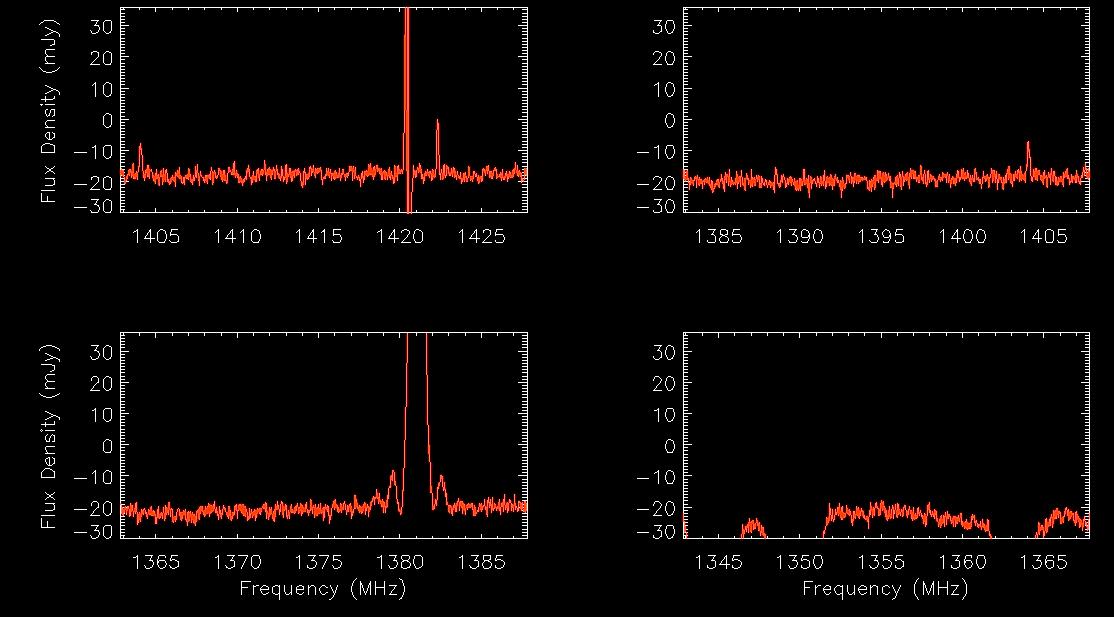
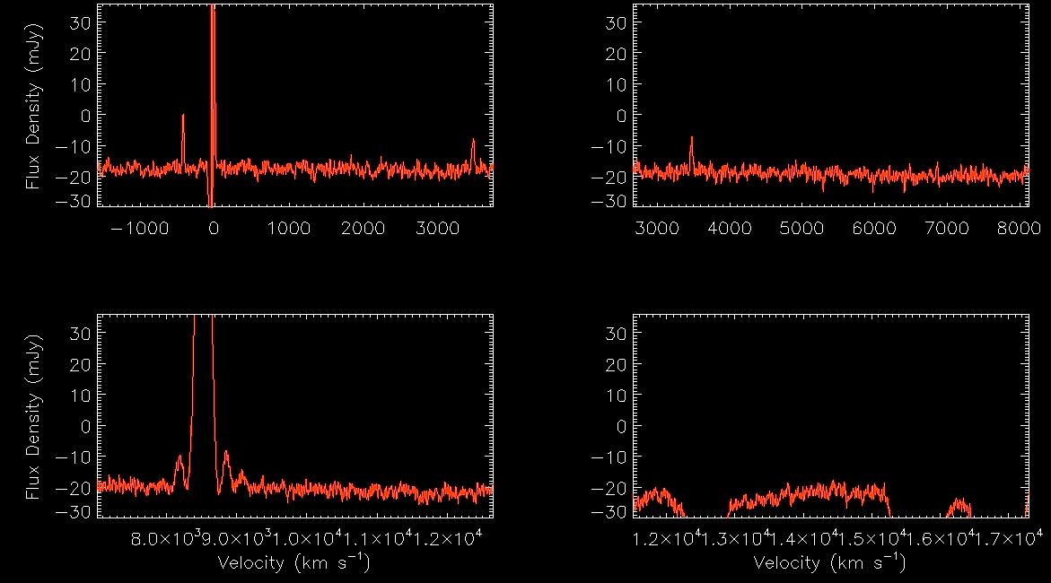
To the right are the four WAPP spectra obtained from the position switched observations of
the galaxy AGC 310858 displayed with the
horizontal axis in frequency units (top) and then velocity units (bottom). Here, the
ON and OFF-source spectra have been differenced and normalized and the calibration derived
from the CAL-ON/OFF sequence has been applied. In the frequency units plots,
there are interesting positive flux density signals (which we designate by letter)
at 1422.3 MHz (A), 1420.4 MHz (B), 1404 MHz (C),
1381 MHz (D); the 4th spectrum covering the lowest frequency range appears quite different.
Let's try to figure out what these spectra show. a. Identify each of the features A, B, C and D in the spectra shown in velocity units. Click here to see a larger version of the first WAPP spectrum, centered at 1415 MHz. b. How can you explain Feature A? c. What is feature B associated with and why does it appear to be show both positive and negative flux density? Click here to see a larger version of the third WAPP spectrum, centered at 1375 MHz. d. Feature D arises from well-known radio frequency interference (RFI). Check out Phil Perillat's list of RFI frequently seen at Arecibo and our own ALFALFA team RFI page. What is Feature D? e. Why isn't the transmitter responsible for the RFI at 1381 MHz on all the time? Hint: See our ALFALFA team RFI page. |
|
|
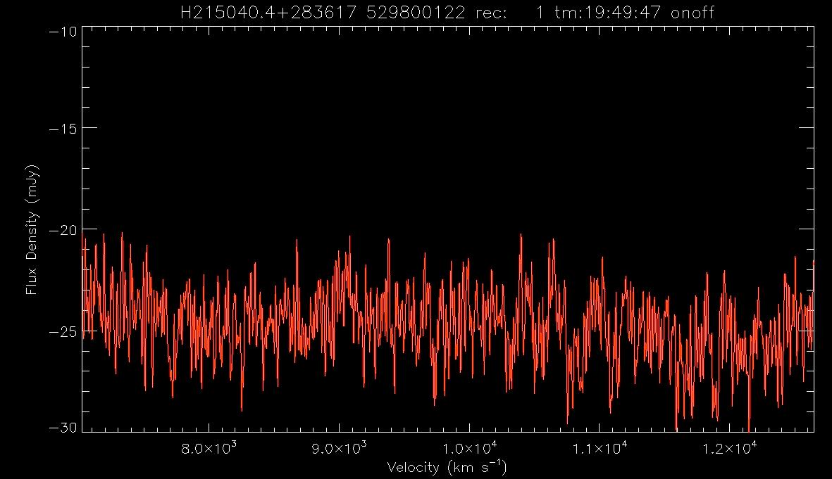
Because the RFI transmitter isn't on all the time, we can discard that portion of the
dataset when it is on to produce an RFI-free difference spectrum; because it contains fewer data records,
it will be noiser that one that contained a full 5 min-ON and 5 min-OFF source but it's better than the one contaminated
with the RFI or having no spectrum at all.
The spectrum to the right shows the result of forming the final spectrum after excising the
records with the RFI present.
f.
Was the transmitter associated with the 1381 MHz RFI on during the ON-source
or the OFF-source portion of the position-switched observations of AGC 310858? Click here to see a larger version of the fourth WAPP spectrum, centered at 1355 MHz. g. What RFI makes the fourth spectrum useless to us? |
|
h. We (finally!) identify Feature C with the target galaxy AGC 310858. Why does it appear in more than one spectrum?
Here are links to various useful public databases: SDSS DR 9, SDSS DR 12, DSS2 Blue, and NED. Be sure you understand what each site contains and how to use/interpret the information/images posted there. AGC 310858 2150403+283527 327.6679 28.5908 DR9Navi DR12Navi DSS2blu.03 NED1.0 i. What do you conclude about the nature, distance, morphology, stellar and gas content of AGC 310858?
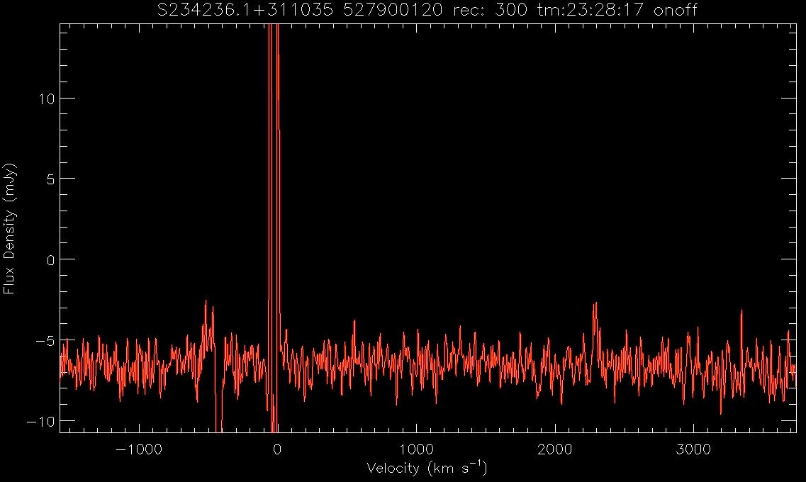
1.5 Interpreting LBW spectra taken in APPSS search mode Use what you have learned above to interpret spectra of targets observed under Arecibo program A2982 in the fall of 2015 under the UAT APPSS program. Below are some of the spectra of AGC 335430, an APPSS target, as well as links to the optical databases as above. In all cases of the images, a larger version will open in a new window if you click on the spectrum
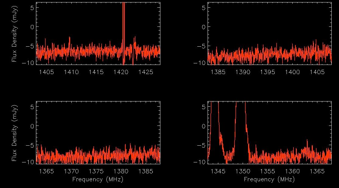 |
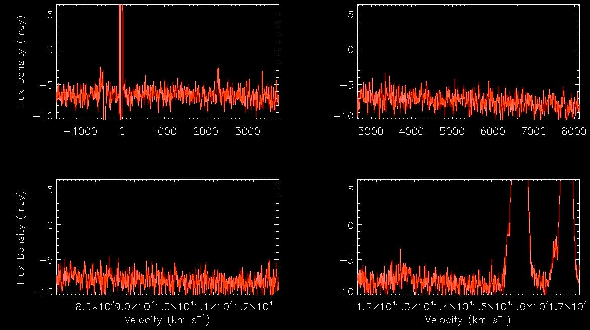 |
 |
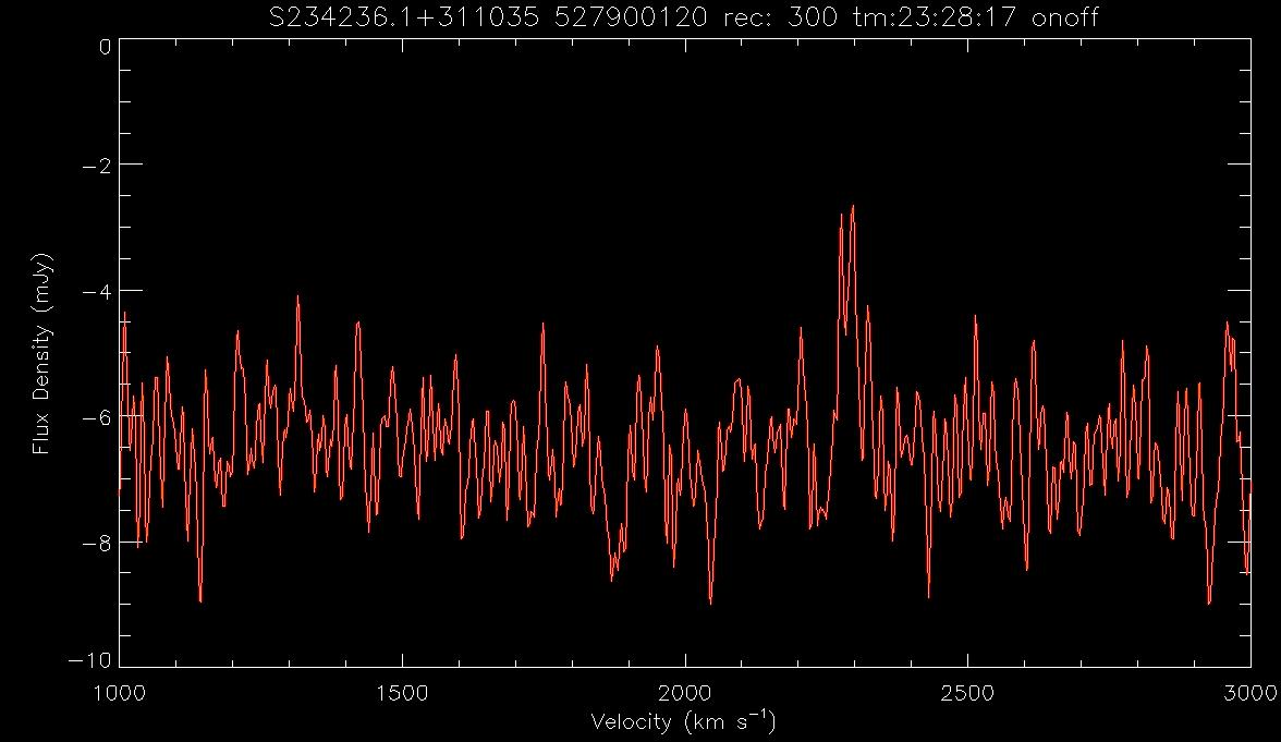 |
Keep in mind that stronger HI sources would have been detected in the ALFALFA survey, so most of the LBW targets should have relatively low integrated HI fluxes.
1.6 ALFALFA Team Trivia: Part II (Some of us think this is important too!)
a. In what 1984 movie did the unsympathetic government agent say: " Do you seriously expect me to tell the President that an alien has landed, assumed the identity of a dead housepainter from Madison Wisconsin and is presently out tooling around the countryside in a hopped up orange and black 1977 Mustang?" b. In the movie "Some Like It Hot", who (what actor) utters the famous closing words "Well, nobody's perfect."? c. What is the temperature at which paper burns, according to the famous futuristic 1967 film starring Julie Christie and Oskar Werner? d. What is odd about the rotation of Venus, and how and when was that determined?
This page created by and for the members of the ALFALFA Survey Undergraduate team Last modified: Sat Jun 11 09:42:12 EDT 2016 by martha