GBT Remote Observing Training for UAT

June 19-21, 2019

GBTIDL Tutorial

To reduce and analyze spectral line data from the GBT, we use a package called GBTIDL. This contains a collection of programs that run in IDL, which is generally available in Green Bank. The package is fully documented at http://gbtidl.nrao.edu/.

For this activity, you will learn how to reduce data using the observations that were made on Pisces-Perseus galaxies at the last UAT workshop.

1. Connecting to a data reduction machine.

a. There are numerous machines in Green Bank that you can use remotely to reduce your data. They are listed at the bottom of the following webpage: http://www.gb.nrao.edu/pubcomputing/public.shtml.

b. You will be doing reduction via a VNC session, so you will need to set up a server on one of these machines. There are instructions on how to do this for remote observing at: https://science.nrao.edu/facilities/gbt/observing/remote-observing-with-the-gbt. Here is a short recap:

i. From offsite, you will ssh to ssh.gb.nrao.edu (you can skip this command if you are in GB). Then you can ssh to one of the data reduction machines, for this example I will use planck (replace this with the actual machine name if on a different machine).

ii. On planck, at the prompt (>) type:

> vncserver –geometry AxB

where A and B are the number of pixels in the desktop you are creating; they should be less than the number on your monitor. Note the number, N, of the VNC session that was created. The first time you do this, you will need to create a vnc password. This should be different from your account password as you may want to share this with other people.

iii. You can then logoff of both planck and ssh.gb.nrao.edu.

iv. If you are offsite, type the following command from a Terminal window: > ssh -L 590N:planck.gb.nrao.edu:590N username@ssh.gb.nrao.edu. This sets up a ssh tunnel allowing you to connect to a VNC session on a machine that you cannot directly access offsite. If you are onsite, you can skip this step.

c. Once you have your VNC session started and your ssh tunnel setup (if needed), you can use a VNC viewer on your computer. If you have a ssh tunnel, you will connect to: localhost:590N. If you do not, then you would connect to: plack:590N.

2. You now should have a desktop that looks something like this:

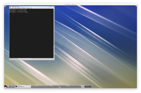
You can interact with this window just like you would on any Linux desktop. If you lose your connection, this window and all its processes will continue to run. Therefore, when you are done with your work, you should login to planck and type > vncserver -kill :N. This will terminate your VNC session and all processes running in it. It is particularly important to exit IDL when not using it as there are a limited number of IDL licenses available in Green Bank.

3. There are three ways to find your data.

a. When looking at data during observing, you can type > online from within GBTIDL.

b. For recent data this can be found in: /home/gbtdata. For our data, we will find it at /home/archive/science-data/17A/AGBT17A_404_01. To get these data into your local directory in the right format, type: > sdfits path (where path is the directory where your data is). For storing large data files, you will want a directory on the scratch disk. Email helpdesk@gb.nrao.edu to request one (when needed).

c. The second (easier) way to access your data is within GBTIDL using the command: > offline,'AGBTX_Y_Z' where X is the semester (17A), Y is the project code (404), and Z is the observing session (01). This method only works for recent observations. We will not do this here.

4. To run GBTIDL, at the system prompt type: > gbtidl

5. You will then need to load your data file. If you used option one above, just type: > filein, filename where filename is the full path of the file you created with sdfits. Alternatively you can leave off the filename and navigate to your file via a GUI. For this work, type: > filein,'/home/scratch/dpisano/GBT17A-404/AGBT17A_404_01.raw.vegas'

6. At this point you can type > summary to see a listing off all the scans from your observation. There are three types of scans in this observation:

a. Observations of a known flux calibrator: 3C48 in this case.

b. Observations of known HI sources, these allow us to confirm that our data reduction is yielding results consistent with past work.

c. Observations of unknown HI sources. These are for doing science.

7. The first step is to determine the appropriate flux scale. To do this, we will use our flux calibrator to derive the temperature of our noise diode, Tcal, in both polarizations. You will type the following commands:

a. > .compile scalUtils

b. > .compile scal

c. > createCalStruct

d. We can then derive Tcal using 3C48 with the following commands:

i. >scal,1,2,tau=[0.01],ap_eff=0.657,plnum=0 (for YY pol)

ii. >scal,1,2,tau=[0.01],ap_eff=0.657,plnum=1 (for XX pol)

iii. The second number printed out when running scal is Tcal for that polarization averaged over the entire bandwidth. We can check that this looks reasonable by typing: > plotCalDB. This will plot Tcal for every channel and print out the average Tcal values. You should get a result for plnum=0,1 of Tcal=1.61,1.65 (respectively). Check if you get a similar result for scans 75, 76. You will want to use the values from the latter two scans.

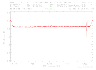
e. Now we can calibrate and reduce the data for each of the galaxies. For starters, pick one. I will use the first of the known HI sources:

i. getps,3,tau=0.01,ap_eff=0.657,units='Jy',tcal=1.61,plnum=0 (you will want to change the italicized numbers to match the values you derived/chose). You should get something that looks like this:

ii. If this looks good, type > accum.

iii. Then repeat for plnum=1 with the appropriate tcal value. If this is also good, type > accum.

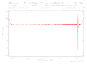
iv. Now type: > ave to get the average of the two polarizations. You should see "Pol: I" printed in the header now, and something that looks like this:

v. This spectrum needs to be baselined. You would start by using setregion, where you will have you click on the line-free regions for subtracting the baseline. You could also set the region by hand using nregion. You should next choose a baseline order with the command: > nfit,1 where 1 is the order. The baseline command will then subtract the baseline.

vi. Congratulations you now have a calibrated HI spectrum of a galaxy!

f. There are a number of additional things you can do with your spectrum now.

i. You can zoom in on the galaxy by using the mouse and cursor to select a region or manually setting the x and y ranges with setx and sety (using the current units on the plotter).

ii. You can switch the units on the x-axis with freq, chan, or velo. Or you can use the drop-down menu on the plotter.

iii. To measure the noise in your spectrum you can use stats.

iv. To smooth your data, you can use boxcar or gsmooth.

g. When you are happy with your results, you can save your spectrum in one of 3 ways:

i. Create an output file using > fileout,outputfile followed by > keep.

ii. You can save the plotter output using > write_ps,psfile

iii. Or you can output the spectrum as a text file using > write_ascii,textfile.

Try this for a few galaxies. Good luck!