Try to finish this activity by 8 pm on Wednesday evening


Rules of the scavenger hunts:   (0): These are scavenger hunts, not tests. Don't expect all the answers to be obvious or google-able. (1): In all cases, return attendees shall not reveal the answers to first timers until sufficient effort is expended. (2): Any bribes must be shared 50:50 with the Scavenger Hunt creators. (3): You may consult any source anywhere but please be sure to indicate where you got your information. And watch out for bad websites! Actually, if you find any mis-information, make a note of it and report to Martha and Becky.


UAT2019 Scavenger Hunt #1:   Using Arecibo and the GBT for UAT HI Line Observations and an Introduction to some of our favorite databases

This scavenger hunt will explore some details of the HI spectral observations we are conducting for the Arecibo Pisces-Perseus Supercluster Survey (APPSS) and the observations we will be doing at Green Bank during this workshop.


1.0   Position-switched observing with single dish telescopes

ALFALFA itself was a "blind drift scan" survey in which we positioned the Arecibo telescope on the meridian, pointed it at a particular declination, started taking data and let the sky drift by. For our APPSS and GBT observations, we point the telescope towards targets identified by the optical and UV emission. The HI line signals that we are trying to detect are billions of times weaker than the radio noise contributed by the radio receiver, the electronics, the antenna, the cosmic microwave background and the sky overall. So, somehow, we have to subtract off all of those unwanted contributions to find the HI signal from the target galaxy. We can do this by assuming that any random position in the sky does not contain an HI line source at the exact same velocity as our target source and that the difference between the spectra obtained in the direction of our target and some suitably chosen random position will yield the signal we are after. The mode of observing we use for the L-band observations is called position switching, where we switched between "ON source" and "OFF source" positions. Thus each observation is actually an ON/OFF pair of observations. Review with your group this link to L-band wide (LBW) observing for ALFALFA followup and APPSS.

    a.   What do we mean by system temperature?


    b.   What is the typical system temperature of the Arecibo L-band receiver system?


    c.   What is the typical system temperature of the L-band receiver system on the GBT?


    d.   Why is the GBT able to deliver a lower system temperature on its L-band system than Arecibo can?


    e.   For our Arecibo position-switched observations for APPSS, a source with a peak flux density of 30 mJy per spectral channel would be easily detected. How does 30 mJy compare with the system temperature you found above?


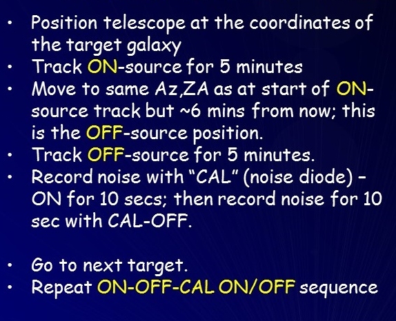
We also need a way to figure out the intensity calibration of the system noise. At the GBT, we observe a continuum source (quasar) at the start of the observing run. At Arecibo, we inject the noise from a diode (whose noise has been measured by the engineers in the lab) into the system and also record the noise when the diode is "off". This sequence is referred to as the "CAL ON/CAL OFF" sequence; we perform this measurement at the end of every target galaxy position-switched ON/OFF pair. A single observation of an APPSS target source then includes both the ON/OFF source observation and the CAL ON/OFF calibration sequence, as summarized by the panel to the right.

Often we observe a source more than once, often on a different day, for example, if there is a marginal detection whose reality we would like to confirm. It is possible to combine multiple observations of the same source to improve the signal-to-noise ratio.

Useful links related to Arecibo observing:

  • Using Arecibo for ALFALFA
  • Using ALFALFA for science
  • A2010 observer's page
  • Observing checklist for LBW observing
  • L-band wide (LBW) observing for ALFALFA followup
  • Standard ALFALFA LBW followup observing modes
  • Instructions on reducing LBW data using IDL_LBW to analyze Arecibo L-band wide spectra taken for ALFALFA followup programs


  • 1.1   The galaxy hosting the HI signal

    Our observations are directed towards detecting the radio HI line signal from the target galaxies, and we also need to understand the stellar population associated with the HI gas. In SH #0, we used links to the public databases of SDSS, SkyView/DSS and the NED. Here we'll provide you with links that you can use to explore some interesting galaxies. Here are links to the front pages of the SDSS, SkyView/DSS and the NED: If you are not already familiar with these really useful websites, we suggest that you should become more familiar with them while you are at and after you return from the workshop. Here, we'll hope that someone in your group knows enough to use them to answer the questions below about some interesting galaxies.

    Consider Object #1:
        a.   This object has lots of cross-identifications. What do "UGC", "CGCG", "MCG" and "2MASS" refer to?

        b.   What is the recessional velocity given by the SDSS spectrum?

        c.   ALFALFA measures a heliocentric velocity of the HI from this galaxy of 5495 km/s. Comment on the comparison with the SDSS value.

        d.   What spectral classification (as given on the image of the spectrum) is assigned to this galaxy by the SDSS? What is the classification based on?


    Consider Object #2:
        e.   How does this object compare with Object #1 as a target for SDSS spectroscopy?

        f.   What spectral classification (as given on the image of the spectrum) is assigned to this galaxy by the SDSS? What is the classification based on?

        g.   How does the SDSS spectrum of this object compare with that of Object #1

        h.   The ALFALFA database lists this as a "Code 2" signal with a recessional velocity from the HI spectrum of 5483 and a signal-to-noise ratio of 4.9. What is a "Code 2" ALFALFA source?


    Consider Object #3:
        i.   What is the best SDSS name to identify with our LBW target (Obj #3)? Why isn't this a trivial question?

        j.   This galaxy is not an SDSS spectroscopic target. Is that a surprise?

        k.   Is a redshift available from NED for this object?

        l.   The ALFALFA database lists this as a "Code 4" signal with a recessional velocity from the HI spectrum of 5862 and a signal-to-noise ratio of 5.8. What is a "Code 4" ALFALFA signal?


    Consider Object #4:
    This galaxy was detected in our current Green Bank observing project at a heliocentric recessional velocity of 2275 km/s on Feb. 23, 2019.

        m.   Compare the SDSS view of this galaxy to the red and blue DSS views. Which is best at detecting the galaxy? Why might this be?

        n.   What other survey provides data for this galaxy?

        o.   This galaxy is part of a sample of very low surface brightness galaxies discovered in the Hyper-Subprime Camera (HSC) survey (Greco et al. 2018 ). A deep image from the HSC survey can be found in this set of example images.   Comment on the shape of this galaxy in comparison to the others you have looked at.

        p.   How does the size of this galaxy compare to that of the Milky Way?


    1.2   Using TOPCAT to match two catalogs

    We hope that you have already had a chance to play with TOPCAT; here we have designed a quick exercise to show how you can use it to match entries in two catalogs. Here are two files for you to work with:
    HI positions and OC positions

    The first one contains a long list of the HI positions of ALFALFA detections; the second one contains the optical coordinates of a subset of the first. Use these two files to answer the questions below. If you have not used TOPCAT before, check out the links given in 0.0 in SH#0.

        a.   How many objects are contained in each of the two catalogs?

        b.   How does the sky distribution of the first set (HIpos) compare to that of the subset (OCpos)?

        c.   Crossmatch the two catalogs by AGC number; use the "Joins" function with the "Pair Match" option and "Exact Value" algorithm in TOPCAT. How many matches do you get?

        d.   Going back to the original catalogs, make a crossmatch using the "Sky" algorithm. Why don't the positions match exactly? How large must "Max Error" be to get the same number of matches that you found when you cross matched by AGC number? Explain your answer.

        e.   What is the mean separation between the HI and OC positions? What is the median value?   Hint: Think about which of the cross-matched catalogs you should use for this; some of them already include the separation. And, you should be able to find the mean and median values easily using built-in functions; ask for advice if you get stuck here.

        f.   For the 2nd file, make a plot of HI mass versus distance. Examine the result and comment on it.


    1.3   The color-magnitude diagram and how galaxy color correlates with morphology

    Probably you are familiar with the Hertzsprung-Russell diagram for stellar classification. We can make a similar "color-magnitude" diagram for galaxies using TOPCAT and the photometric data from the SDSS. For nearby galaxies, there are problems with the standard SDSS photometric pipeline, so we use the ones available through the NASA-Sloan Atlas (N-S Atlas). We can also look at the morphological classification provide by the citizen science project Galaxy Zoo.

    For this exercise, we have put together a useful dataset in CSV format from a combination of the N-S Atlas and the Galaxy Zoo 1 data release. It does not cover the whole sky because each galaxy has to be included in both catalogs. The file contains the basic information plus we have calculated a color (called "gminusi") and an absolute magnitude ("absmagi") as well as an indicator of morphology. Note that the way the morphological type is identified is by having a flag set to "1" according to whether the galaxy was classified as "spiral", "elliptical" or "uncertain". In fact, most galaxies are typed "uncertain".

        a.   Why do we call the difference between the magnitude measured in the SDSS-g band and that in the SDSS-i band a "color"?

        b.   Because we wanted to keep things simple, using only the raw data as they are included in the compilations, we have limited this subset to galaxies which are viewed face-on. Why does that make things simpler?

        c.  First, using the N-S Atlas magnitudes, make a color-magnitude diagram using the absolute magnitude and color given here. Be sure that luminosity increases from left to right and that blue galaxies are towards the botton, red towards the top. What do you notice about the distribution of galaxies?   (Note: this diagram will be useful to some of the teams in SH#3).

    Next, let's add the information about morphology from the GZ.

        d.   Use the "column statistics" capability to figure out quickly the fraction of the galaxies which are classified as ellipticals? As spirals? As uncertain?

        e.  Using the TOPCAT subsets capability, plot the spirals and ellipticals separately, using different symbols/colors. Superpose the spirals on the ellipticals (be sure to do it in that order). What do you conclude?


    1.4   The Pisces-Perseus Supercluster

    Filamentary structures are predicted to be pervasive throughout the cosmic web, but they have received relatively little observational attention in comparison to other cosmic overdensities such as clusters. The Pisces-Perseus Supercluster (PPS) forms a strong linear density enhancement, stretching more than 50° across the Arecibo sky. This filament is fortuitously oriented perpendicular to the line-of-sight and separated from surrounding structures by foreground and background voids. PPS serves as a laboratory for studies of how the HI content of galaxies may vary depending on the location of a galaxy within its large scale structure. Because it is a strong overdensity in the local universe, galaxies in its foreground and background should be gravitationally pulled towards it, inducing "peculiar velocities" of infall and backflow onto their Hubble flow velocities.

        a.   Use the NASA Astrophysics Data System (ADS) bibliographic service to find the (ancient and honorable) paper on the PPS by Wegner, Haynes & Giovanelli (1993; Astron.J. 105, 1251). If you have never used the ADS abstract server before, take the opportunity to learn how to use it now. It will find you scholarly references that Google and Wikipedia won't necessarily.

        b.   What is the epoch in which coordinates are presented (e.g. Table 1) in this paper? What does "coordinate epoch" refer to and why do we have to pay attention to this detail?


    The figure below shows the distribution of galaxies with known recessional velocity (abbreviated as cz, with cz <12000 km/s here) in a wide area of sky around PPS. The superposed dark lines outline the region of the main ridge of the PPS.

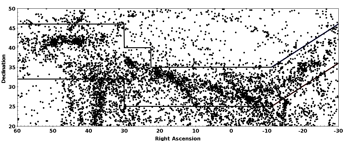
        c.   Which figure in the Wegner et al. paper is similar to this figure? What is different about the one displayed here?


        d.   Why do we display Right Ascension increasing towards the left?


        e.   Draw on the diagram the northern declination limit of the Arecibo telescope.

    The figure below also resembles (deliberately) a figure presented in the Wegner et al. paper. Take note of the similarities and differences.

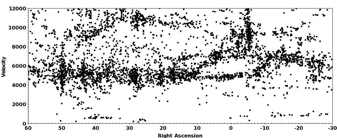
        f.   What do we mean by "heliocentric velocity"?


    The table below, based in large part on Table 3 of the Wegner et al. paper, lists the main galaxy groups and clusters associated with PPS.

    Name Common Name R.A.(J2000)
    (deg)
    Dec(J2000)
    (deg)
    cz
    (km/s)
    N7343 Pegasus 339.7 34.0   6000.
    Abell 2634   354.6 27.0   9400.
    Abell 2666 Pegasus 357.7 27.2   8000.
    N 383 Pisces 16.9 32.4   4800.
    N 507   20.5 33.3   4700.
    Abell 262   28.2 36.2   4800.
    Abell 347   36.5 41.9   5600.
    Abell 426 Perseus 49.7 41.5   5500.

    Note: The values in the above table are taken various sources (including the Wegner+ paper) and have been rounded off; we should derive new ones someday using the ALFALFA and APPSS data and any other more recent data taken from the literature.


        g.   Mark and label each of the groups/clusters on the two Figures above.


        h.   Discuss your impressions of the PPS within your group. Make a mental picture of PPS and keep it in mind when we discuss the APPS Survey. We'll return to PPS in later Scavenger Hunts.


    1.5   ALFALFA Team Trivia: Part II   (Some of us think this is important too!)

    a.   In what 1984 movie did the unsympathetic government agent say: " Do you seriously expect me to tell the President that an alien has landed, assumed the identity of a dead housepainter from Madison Wisconsin and is presently out tooling around the countryside in a hopped up orange and black 1977 Mustang?"

    b.   In the movie "Some Like It Hot", who (what actor) utters the famous closing words "Well, nobody's perfect."?

    c.   What is the temperature at which paper burns, according to the famous futuristic 1967 film starring Julie Christie and Oskar Werner?

    d.   What is odd about the rotation of Venus, and how and when was that determined?


    1.6 (Extra)   HI emission from the Milky Way itself

    The Milky Way Galaxy contains about 3 x 10⁹ solar masses of HI. We detect it in all of the Arecibo spectra (and would if we used a much smaller telescope too!).

        a.   Where is most of the neutral atomic hydrogen in the Milky Way found?


        b.   At what velocities should we expect to see HI emission from the Milky Way?   Hint: refer back to SH #0.


        c.   What is a High Velocity Cloud?


        d.   What is the recessional velocity of Andromeda (Messier 31)?


        e.   What is the recessional velocity of the Triangulum Galaxy (Messier 33)?


        f.   What is the recessional velocity of Leo P?


    This page created by and for the members of the ALFALFA Survey Undergraduate team

    Last modified: Fri Jun 14 07:33:38 EDT 2019 by becky