
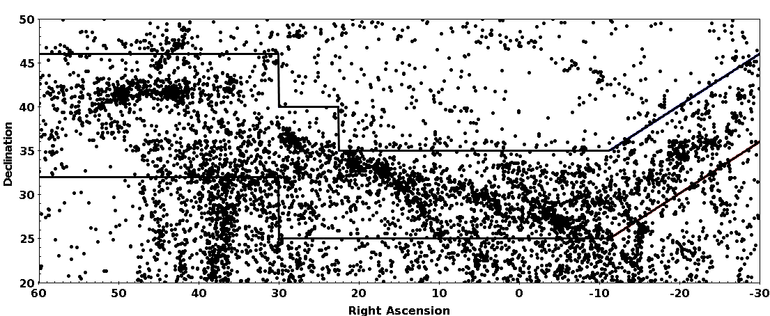
 c. Which figure in the Wegner et al. paper is similar to this figure?
What is different about the one displayed here?
c. Which figure in the Wegner et al. paper is similar to this figure?
What is different about the one displayed here?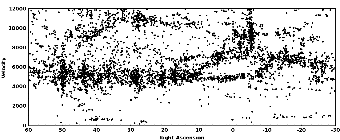 f. What do we mean by "heliocentric velocity"?
1.1 Position-switched observing with single dish telescopes ALFALFA itself was a "blind drift scan" survey in which we positioned the Arecibo telescope on the meridian, pointed it at a particular declination, started taking data and let the sky drift by. For our APPSS observations, we point the telescope towards targets identified by the optical and UV emission. The HI line signals that we are trying to detect are billions of times weaker than the radio noise contributed by the radio receiver, the electronics, the antenna, the cosmic microwave background and the sky overall. So, somehow, we have to subtract off all of those unwanted contributions to find the HI signal from the target galaxy. We can do this by assuming that any random position in the sky does not contain an HI line source at the exact same velocity as our target source and that the difference between the spectra obtained in the direction of our target and some suitably chosen random position will yielf the signal we are after. The mode of observing we use for the L-band wide observations is called position switching, where we switched between "ON source" and "OFF source" positions. Thus each observations is actually on ON/OFF pair of observations. Review with your group the link noted above: L-band wide (LBW) observing for ALFALFA followup. a. What do we mean by system temperature?
b. What is the typical system temperature of the Arecibo L-band receiver system?
c. What is the typical system temperature of the L-band receiver system on the GBT?
d. What is the GBT able to deliver a lower system temperature on its L-band system than Arecibo can?
e. For our Arecibo position-switched observations for APPSS, a source with a a peak flux density of 30 mJy per spectral channel would be easily detected. How does 30 mJy compare with the system temperature you found above?
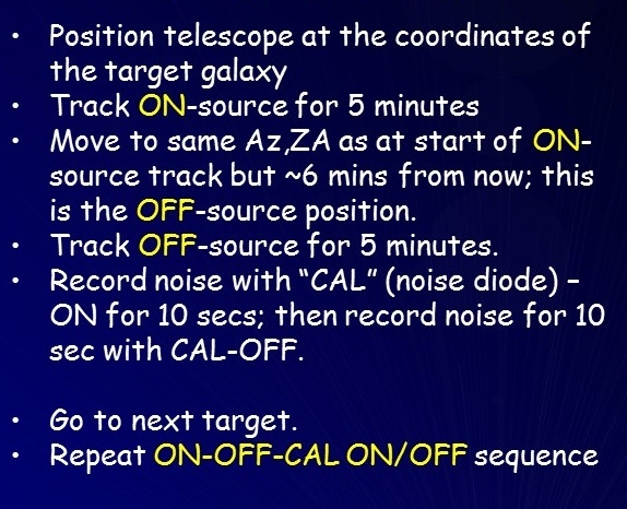
| We also need a way to figure out the intensity calibration of the system noise. To do this, we inject the noise from a diode (whose noise has been measured by the engineers in the lab) into the system and also record the noise when the diode is "off". This sequence is referred to as the "CAL ON/CAL OFF" sequence; we perform this measurement at the end of every target galaxy position-switched ON/OFF pair. A single observation of a target source then includes both the ON/OFF source observation and the CAL ON/OFF calibration sequence, as summarized by the panel to the right. Sometimes, we observe a source more than once, often on a different day, for example, if there is a marginal detection whose reality we would like to confirm. It is possible to combine multiple observations of the same source to improve the signal-to-noise ratio. |
|
1.2 Searching for galaxies using L-band wide You may have noticed that the "spectrometer" described in our webpage L-band wide (LBW) observing refers to a different spectrometer than we actually use when we "search" for galaxies. Some of one these days, we ought to update that page... Here we'll investigate the spectral setup we use to "search" for HI line emission from galaxies whose redshifts we do not know. A major component of the UAT APPSS program includes observations with the Arecibo telescope to detect HI line emission from galaxies which, based on their optical properties in the Sloan Digital Sky Survey (SDSS) and Galaxy Explorer (GALEX) databases, are likely members of the supercluster or its immediate foreground/background. We'll talk about how we select targets for the HI observations later. For now, let us focus on how we conduct the Arecibo observations using the L-band wide receiver system. For this part of the exercise, review the WAPP search mode documentation. a. What does "WAPP" stand for?
b. How many WAPP boards are there?
c. In Scavenger Hunt #0, we reviewed the definition of redshift, z, in terms of wavelength; this relation Δλ/λ is sometimes referred to as the "optical" definition of redshift, while the "radio" expresses redshift in terms of Δf/frest, where Δf is the difference between the observed and rest frequency of the line emission. In order to be consistent with redshift (or recessional velocity) measurements made at different wavelengths, we use the "optical" definition. Work out for yourself the relationship between z, fobs and frest under the optical definition.
d. In the WAPP "search mode", we divide the spectrometer into four quadrants, each of which produces a spectrum covering 25 MHz. Their center frequencies are offset one from the other by 20 MHz. Why do we overlap the frequency range of the quadrants?
e. In this setup, what at is the total velocity range of the combined WAPP coverage?
f. We refer to each frequency "pixel" as a "channel": there are 2048 channels for each 25 MHz. The center frequencies of each channel are spaced by a constant δf = 25 MHz/2048 channels. What does this imply for the separation of channels if we convert them to velocity units (km/s)?
1.3 HI emission from the Milky Way itself The Milky Way Galaxy contains about 3 x 10⁹ solar masses of HI. We detect it in all of the Arecibo spectra (and would if we used a much smaller telescope too!). a. Where is most of the neutral atomic hydrogen in the Milky Way found?
b. At what velocities should we expect to see HI emission from the Milky Way? Hint: refer back to SH #0.
c. What is a High Velocity Cloud?
d. What is the recessional velocity of Andromeda (Messier 31)?
e. What is the recessional velocity of the Triangulum Galaxy (Messier 33)?
f. What is the recessional velocity of Leo P?
1.4 Using TOPCAT to match two catalogs We hope that you have already had a chance to play with TOPCAT; here we have designed a quick exercise to show how you can use it to match entries in two catalogs. Here are two files for you to work with:
The first one contains a long list of the HI positions of ALFALFA detections; the second one contains the optical coordinates of a subset of the first. Use these two files to answer the questions below. If you have not used TOPCAT before, check out the links given in 0.0 in SH#0. a. How many objects are contained in each of the two catalogs? b. How does the sky distribution of the first set (HIpos) compare to that of the subset (OCpos)? Crossmatch the two catalogs by AGC number; use the "Joins" function with the "Pair Match" option in TOPCAT. How many matches do you get? c. Going back to the original catalogs, make a crossmatch using the "Sky" algorithm. Why don't the positions match exactly? How large must "Max Error" be to get the same number of matches that you found when you cross matched by AGC number? Explain your answer. d. What is the mean separation between the HI and OC positions? What is the median value? Hint: Think about which of the cross-matched catalogs you should use for this; some of them already include the separation. And, you should be able to find the mean and median values easily using built-in functions; ask for advice if you get stuck here. e. For the 2nd file, make a plot of distance versus HI mass. Examine the result and comment on it.
1.5 The color-magnitude diagram and how galaxy color correlates with morphology Probably you are familiar with the Hertzsprung-Russell diagram for stellar classification. We can make a similar "color-magnitude" diagram for galaxies using TOPCAT and the photometric data from the SDSS. For nearby galaxies, there are problems with the standard SDSS photometric pipeline, so we use the ones available through the NASA-Sloan Atlas (N-S Atlas). We can also look at the morphological classification provide by the citizen science project Galaxy Zoo. For this exercise, we have put together a useful dataset in CSV format from a combination of the N-S Atlas and the Galaxy Zoo 1 data release. It does not cover the whole sky because each galaxy has to be included in both catalogs. The file contains the basic information plus we have calculated a color (called "gminusi") and an absolute magnitude ("absmagi") as well as an indicator of morphology. Note that the way the morphological type is identified is by having a flag set to "1" according to whether the galaxy was classified as "spiral", "elliptical" or "uncertain". In fact, most galaxies are typed "uncertain". a. Why do we call the difference between the magnitude measured in the SDSS-g band and that in the SDSS-i band a "color"? b. Because we wanted to keep things simple, using only the raw data as they are included in the compilations, we have limited this subset to galaxies which are viewed face-on. Why does that make things simpler? c. First, using the N-S Atlas magnitudes, make a color-magnitude diagram using the absolute magnitude and color given here. Be sure that luminosity increases from left to right and that blue galaxies are towards the botton, red towards the top. What do you notice about the distribution of galaxies? (Note: this diagram will be useful to some of the teams in SH#3). Next, let's add the information about morphology from the GZ. d. Use the "column statistics" capability to figure out quickly the fraction of the galaxies which are classified as ellipticals? As spirals? As uncertain? e. Using the TOPCAT subsets capability, plot the spirals and ellipticals separately, using different symbols/colors. Superpose the spirals on the ellipticals (be sure to do it in that order). What do you conclude?
1.6 ALFALFA Team Trivia: Part II (Some of us think this is important too!)
a. In what 1984 movie did the unsympathetic government agent say: " Do you seriously expect me to tell the President that an alien has landed, assumed the identity of a dead housepainter from Madison Wisconsin and is presently out tooling around the countryside in a hopped up orange and black 1977 Mustang?" b. In the movie "Some Like It Hot", who (what actor) utters the famous closing words "Well, nobody's perfect."? c. What is the temperature at which paper burns, according to the famous futuristic 1967 film starring Julie Christie and Oskar Werner? d. What is odd about the rotation of Venus, and how and when was that determined?
This page created by and for the members of the ALFALFA Survey Undergraduate team Last modified: Fri Jun 15 11:00:57 EDT 2018 by martha