A Brief Introduction to TOPCAT


  • Link to TOPCAT


    Getting ready for TOPCAT

    TOPCAT is a JAVA utility developed under the auspices of the international "Virtual Observatory" concept which enables the manipulation, display and analysis of datasets, specifically astronomical ones. Please refer to the above link for detailed information and downloading instructions. Note that TOPCAT can be installed on Windows, MacOS and Linux platoforms that are also Java-enabled.

    Here, I assume that you have already installed TOPCAT successfully.


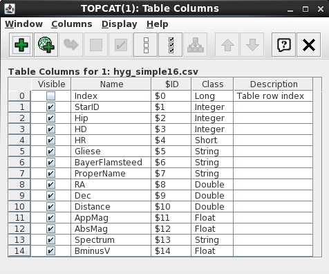
    Getting a dataset for TOPCAT

    Many astronomical datasets are publicly available on the internet. As an introduction to TOPCAT, let's make use of a catalog of 87,000 stars with measured distances, spectra and radial velocities contained in the HYG database at http://wwwtronexus.com/node/34. The database is a subset of data contained in three large catalogs of stars: the Hipparcos Catalog, the Yale Bright Star Catalog, and the Gliese Catalog of Nearby Stars. For convenience, we have made a simple version of the database which you can find here. Be sure you know in what directory it is located after you download it. Now, let's make the plot shown on the right.

  •   Start TOPCAT. On Windows machines, that means clicking on the file "topcat-full" in the directory where you have downloaded the executable jar file of that name. The TOPCAT window will appear.

  •   Click on "File" (upper left) and then "Load Table". A new "Load New Table" window will appear. Choose the appropriate "Format", here "CSV".

  •   Click on "System browser". Find the datafile of stars that you download. Click on it so that its name appears under "File name" at the bottom of the "Load Table" menu. On Windows machines, be sure that the bottom file type says "All Files". Click on "Open" and the file should load. It might take some seconds. The file name should appear in the "Table List".

  •   Left click on "Views" and then "Column Info". A new window will open which lists the Names of each column in the table. Notice what they are.

  •   Back in the main menu, left click on "Graphics" and then on "Plane Plot". A new window will appear. By default, it has plotted column 1 ("StarID") on the X axis and column 2 ("Hip") on the Y axis. What we want however is to plot "BminusV" on the X axis and "AbsMag" on the Y axis. Left click on the downward arrow next to "StarID" and select "BminusV"; then do the same for "AbsMag". This plot should appear.

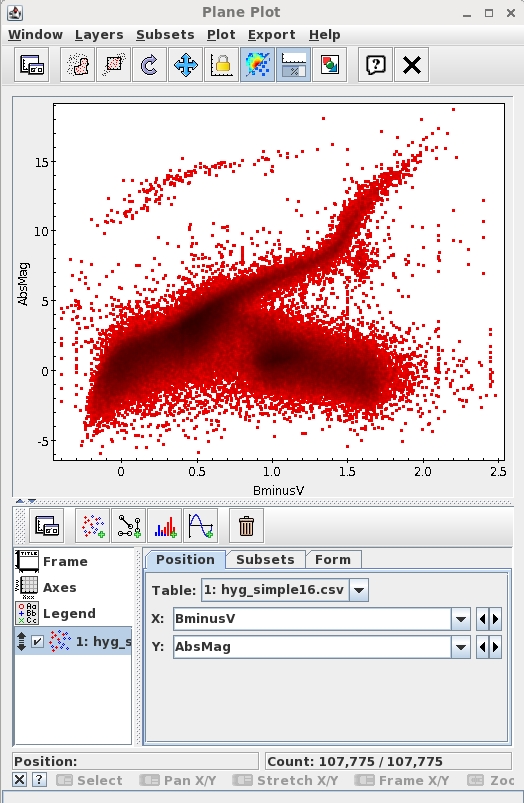
    Notice that it bears some resemblance to the plot we wanted to make (shown above on the right), but (a) the data points appear are denoted by red symbols not black ones, (b) it seems to have the Y axis scale flipped and (c) the range of X and Y values is not what we want. We need to fix those things.

  •   As you may already know, astronomers measure the brightnesses of objects using a system of "magnitudes" that is logarithmin and inverse, that is a larger magnitude means a fainter object. So for our plot, we want to flip the Y axis of the plot. First, click on the "Axes" icon on the left and then click on the small box next to "Y Flip". That looks better!

  •   Next, let's change the color of the data point symbols. Click on the name of the table again and then, on "Subsets". You will see an entry labelled "Color" which is set to red. Click on the down arrow to the right of the red "Color" bar. Scroll down and select the black bar. The color of the points will change!

  •   To finish the job, we need to reset the range of the X and Y values. Click again on "Axes" and then on "Range". In this case, set X range from -0.5 to 2.5 and the Y range to -6 to 16 and then click "Submit"; the plot will rescale.

    Finally, let's add a title to the plot. Click on "Frame" and then on "Title". Enter "Hipparcos Color-Magnitude Diagram" and hit "Enter". You should see:

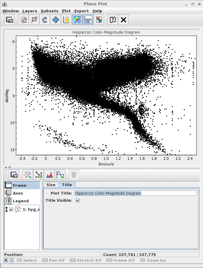
    Notice that some of the points disappear because they lie outside the specified ranges. We'll talk about that later....

  •   As one final step in this example, let's save the plot by exporting a copy to your machine's disk. At the top of the "Scatter Plot" window, left click on "Export" and then "Export as gif" (or other format if you want). A window will open which allows you to specify the file name and directory where it will be saved. When you have specified them, click on "Write gif" and you should now have a copy of the plot you have made. When you open the file, select your browser (or other image display utility) when asked for what program to open it with.

    TOPCAT has many more features, so we invite you to explore its capabilities further. Lots of astronomers use TOPCAT, so you are now in good company!


    Last modified: Thu May 12 18:28:33 EDT 2016 by martha